


CodeWalkthrough: 1 billion rows challenge in Python
My attempt at the 1 billion rows challenge and what it has taught me

I first heard about the 1 billion rows challenge (1brc) on LinkedIn and found it very interesting. Basically, this challenge is about processing 1 billion rows of fictitious measurement data as quickly as possible. The catch is, you can only use functions from the standard library.
As a data scientist, I’m used to reaching out to libraries like Pandas or Apache Spark to do my data processing. It’s almost a reflex. I’ve never really had to do data processing in the raw form. I guess I’m spoiled by the Python ecosystem. So I thought the 1brc might be a good challenge for me to learn about the nuts and bolts of Python that I don’t usually use or take for granted.
In this blog post, I will be writing about my attempts at the 1brc. As usual for my code walkthroughs, I will be posting links to the git repo code for the reader to follow along.
I will also be talking about my failed attempts as I feel that we learn as much from our failures as our successes, if not more.
The 1 Billion Rows Challenge
The 1brc is stated as below according to the website.
Your mission, should you choose to accept it, is to write a program that retrieves temperature measurement values from a text file and calculates the min, mean, and max temperature per weather station. There's just one caveat: the file has 1,000,000,000 rows! That's more than 10 GB of data! 😱
The text file has a simple structure with one measurement value per row:
Hamburg;12.0
Bulawayo;8.9
Palembang;38.8
Hamburg;34.2
St. John's;15.2
Cracow;12.6
... etc. ...
The program should print out the min, mean, and max values per station, alphabetically ordered.
Associative operations are your friends
The first thing to note that the values to be calculated here are the results of associative mathematical operations. What this means is that the order in which the rows are process does not matter. Just like how (a + b) + c = a + (b + c).
In the case of calculating the minimum value, say we have 6 measurements, A, B, C, D, E and F. The minimum of the 6 values can be written as follows,
What this means is that the minimum of the 6 values is the minimum of the minimum of subsets of the 6 values.
The same goes for calculating the maximum value.
This means that we can calculate the minimum or maximum of indidvidual partitions of all the measurements and then calculate the overall minimum or maximum. Basically, we can divide and conquer.
As for calculating the average, we cannot take the average of averages to get the final average since it is not guaranteed that each average value is the result of the same number of samples. However if we look at the formula of an average shown below, we see that an average value consist of the sum of the measurements and the sum of the counts, both of which are associative operations.
This means we just need to keep track of 2 numbers: 1) the total number of samples and 2) the sum of the measurements in this subset of data in order to calculate the final average.
All in all, the calculations required from 1brc can be done using the map-reduce strategy where the large dataset is partitioned into several parts and the values required are calculated independently for each partition before being combined to get the final answer.
The Accumulator class
Realising the above, we can then code an object that helps us implement the map-reduce logic. This is done using the Accumulator class in the code. It is expected to keep track of the statistics from each partition of the data.
The first thing to note is the update method which takes advantage of the associativity of the operations to collate the statistics on sample count, minimum, maximum and sum of all the measurements for each station. This is for the “map” phase of map-reduce.
The second thing to note is the __add__ method. This allows me to add the Accumulators from different partitions together to get the final result. This is for the “reduce” phase of map-reduce.
Attempts at 1brc
I made three attempts at 1brc. The first one was a flop. The second one worked better but no where near the State-of-the-Art (SOTA). The last one was strongly inspired and fundamentally the same as the SOTA.
Attempt 1: Single Queue
Given that I know that map-reduce is the key strategy to be used here, my first attempt was to have a process read the file contents and place it in a single queue to be consumed by multiple workers. I would put the data row-by-row into the queue. This is in the main_singlequeue.py file.
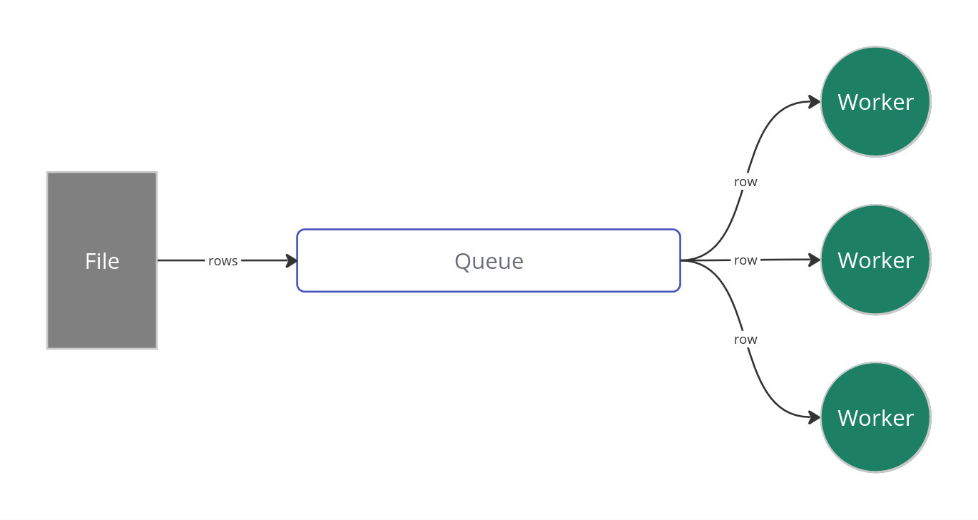
This idea failed quite badly as each time only one worker can pop data off the queue. The problem is made worse as each time only 1 row is obtained from the queue for processing. This means that most of the time the workers are simply waiting around for data as it was very quick to update a single sample.
It took 2 mins to process 4 million samples. Clearly inefficient.
Other things I noted during this attempt is that:
The worker sometimes is unable to obtain data from the queue. Either because data is not being enqueued fast enough or something due to multiprocessing
You can’t pass vanilla multiprocessing queues created using
mp.Queuetoapply_syncin multiprocessing. You need to use amp.Managerto create a queue in a separate thread if you want to useapplyorapply_sync.If you want to get results back from
mp.Process, you need to use something like a dictionary created usingmp.Manager.
Attempt 2: Parallel Queues
Learning from the previous attempt, I thought I would make a few changes.
Instead of putting the data into queues row-by-row, I will instead put batches of rows into the queue each time. This way the workers don’t need to keep getting samples from the queue and can spend more time processing data
I will distribute the samples across parallel queues in a round-robin fashion.
Each queue will only have one worker working on it. In this way, we don’t have multiple workers trying to pop items off the queue at the same time.
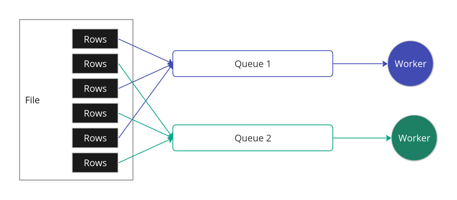
This time it is better, 100 million rows took around 1 min 46s. Still a far cry from SOTA but much better.
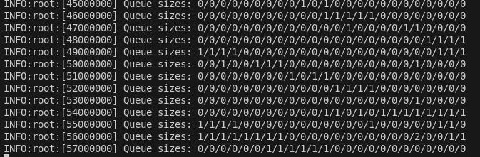
However, this method requires tuning. For example, if the batch size is too small, the workers spend a lot of time simply getting the items from the queue. If the batch_size is too large, the queues will be largely empty as the file reading process can’t fill up all the parallel queues fast enough. See below when a batch size of 10000 was used many of the queues were empty.
Another thing I noticed is that because dequeueing items from the queue takes time, the CPU usage of the workers don’t reach 100 percent. Which means I am not processing as fast as I can.
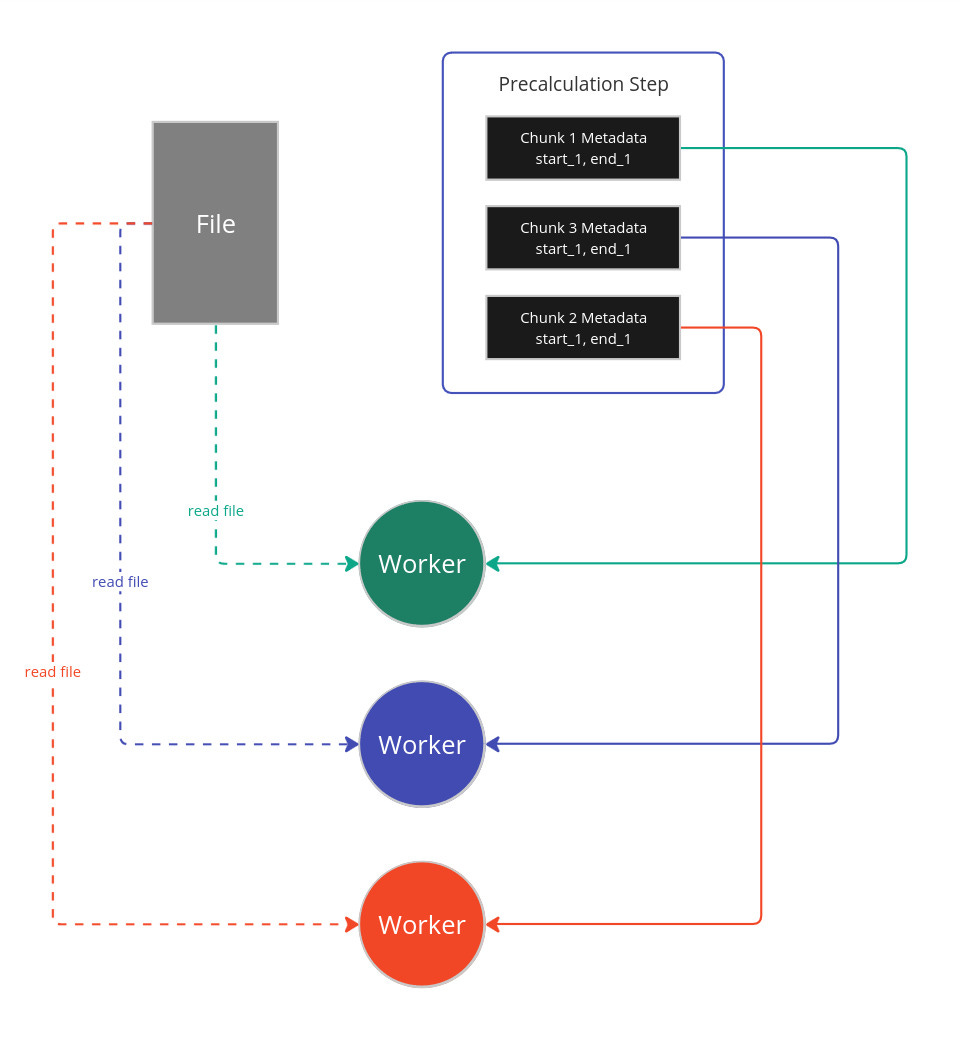
Attempt 3: Prechunking
After attempt 2, I realised that it is very inefficient to send data across the queues like this. So I referenced the published methods to see how they were able to reach such speeds.
Essentially, the map-reduce approach was still used. The collection of data statistics across partitions was still the same as what I did with the Accumulator.
However, what was done differently was that before doing any processing there was a step to prechunk the file into big partitions and to calculate the cursor positions of the start and end of each chunk. Basically, a scan through the file was done to find the byte-position of the start and end of each chunk. So if you intend to distribute the work to 8 workers, you’d have 8 (or 9, depending on whether there are left over rows after dividing by 8) chunks.
This information is then passed to each worker. One chunk to each worker. Note that only the chunk start and end information was passed, not data. Each worker will then independently read the file from it’s respective chunk start and start processing.
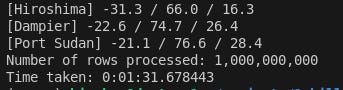
I was able to process 1 billion rows in 1 min 32s.
The thing I found really clever was that only the chunk metadata was used. This made things really fast and the workers are no longer idle while popping data off the queue. My CPU usage was 100 percent.
On top of that, when each worker opens the file using the open function, an iterator is returned. This means that the memory usage is very minimal as we are not loading the whole file into memory. See here and note the “f.seek” line and the “for line in f” line.
A word on the reduce phase
I didn’t put in the reduce phase in the diagrams above as it makes things messy. The process is very simple, I collect the individual accumulators from each worker and add them all up.
Conclusion
All in all this was a fun challenge and helped me understand the workings of Python and multiprocessing a lot more.