Experiment: Structure-from-Motion using COLMAP

Generating 3D structures from 2D images

Structure-from-Motion (SfM) is the process of generating 3D structures via information garnered from a collection of 2D images. In this experiment, I will walk through the use of the COLMAP application to do SfM as well as describe my learnings along the way.

This post is part of my journey to learn about SfM. See related posts here.

Overall process

COLMAP uses a technique that is probably state-of-the-art around 6-7 years ago. I will be experimenting with new techniques such as 3D Gaussian Splatting that have come up in the last couple of years in later posts.

The purpose of going through the use of COLMAP is to how the field came to be and also the fundamental concepts involved such as epipolar geometry.

The first step is to identify good image features that would be easily identifiable from different perspectives. This is done usually via the SIFT or ORB algorithms. For an example of how this is used, see my previous post on image stitching.

The features are then matched across images. The OpenCV website has a great series of tutorials on this. The difficulty here is finding good image pairs to match each other’s features with. A series of techniques/optimizations such as using robust image descriptors are applied here. This is because, the better the matching the better the results in the later steps.

The next step is to find out the camera poses of each image. Basically, what rotation and position relative to the object (or other cameras) is the camera at in the picture. This is done by solving for the fundamental matrix, which is kind of like the homography matrix, using the matched features in the previous step and epipolar geometry. In essence, you figure out what transformations are needed to move the features in one image to the matched feature positions in another. This then gives access to fundamental quantities such as the rotation and translation matrices as well as estimated intrinsic camera parameters (such as focal length).

The depth of the matched features are then found via triangulation. This gives a sparse representation of the 3D structure. Why “sparse”? This is because only the matched feature depths are estimated and not for every pixel in the image. The difficulty here is that the depth of the features have to be globally consistent. All the images must agree.

The last step is dense reconstruction. In COLMAP, an algorithm called PatchMatch to find correspondences between different image patches. Then armed with the rotation and translation matrices and the camera intinsic parameters, the depth and normals of each patch is then figured out. For an explanation of the process see this paper. The normals are important as you can’t just know where the surface is if you want to construct a 3D mesh, you also need to know which direction it is facing. Then with both depth and normal a 3D mesh can be constructed using a process like Poisson Surface Reconstruction.

For detailed explanations, I have found Schonberger’s thesis to be a great resource. I dare not expound in details the inner workings of each step as I am not an expert. My understanding here may not be fully accurate / complete. The description above is simply an attempt to outline the overall process and break a big black box into a series of smaller black boxes according to my understanding.

There are also many variations to the above-mentioned process. Computer vision is a vast field.

As an aside, I had naively wanted to code SfM from scratch initially. That though was quickly vanquished once I saw how complicated the SfM pipeline was and realised that it would months of work before I saw any result. Something I might do if I were doing a postgraduate in Computer Vision (CV) but not as a CV hobbyist.

Experiment Steps

1. Install COLMAP

   1. I built COLMAP from source so that it can utilise my GPU

2. Download test images

   1. In this experiment, I used the “South Building” images

3. Follow instructions in “Quickstart”

   1. The auto-reconstruction mode is pretty straightforward. Simply point COLMAP to your project and image folders

   2. There are more features that can be explored if you want fine-grained control or only want to use certain steps. I didn’t explore too much as I want to move on quickly to Gaussian Splatting.

4. Visualise the results using MeshLab

5. [Optional] Visualise using Blender

   1. The .ply files can be readily imported into Blender.

Results

Processing Time

I didn’t keep exact time but the total processing time for the 128 images in the “South building” dataset took many hours. Most of the time was spent in the dense reconstruction stage. This is one of the reasons why I want to move on quickly to Gaussian Splatting, which only requires the results from the sparse reconstruction and promises quick rendering.

Final output

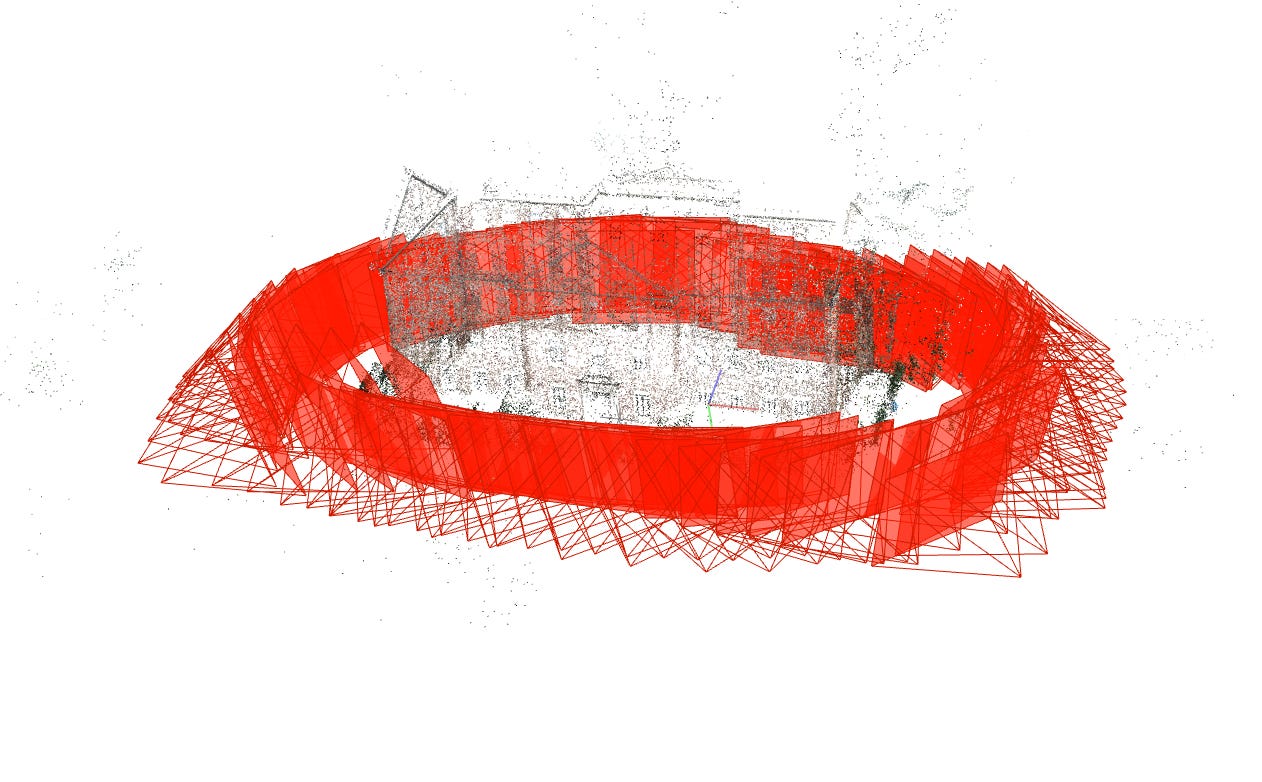
The point cloud from the sparse reconstruction is shown below. It’s really just a collection of points and doesn’t cover every single part of the building.

The red squares are the recovered camera orientations for each of the input images.

After dense reconstruction and Poisson mesh generation, a 3D surface model is generated. This starts to look like something that you would see on Google Maps or a video game in the 2000’s. Note that not all parts of teh building is generated. Parts of the roof, where there isn’t enough information is missing from the generated mesh.

Image requirements

I had initially tried to do the reconstruction with my own images but the generation failed miserably. This is because the object of reconstruction, at least using COLMAP’s SfM pipeline, should be dominant in the images. Just like how the South Building takes up most of the pixel real estate in the images. Otherwise, most of the information will be coming from peripheral objects such as the table the object is on.

One way to circumvent this might be to segment the object out from the background before performing SfM.

Final thoughts

I honestly had no idea what I was getting into when I said I wanted to attempt SfM. If I had, I probably would have picked another topic to explore. Nonetheless, it was refreshing to learn about topics like epipolar geometry and how that could be used to solve for real-world parameters.

In digging deeper about SfM, I’ve also realised that traditional methods, like those demonstrated in OpenCV tutorials, have very high information requirements to begin. For example, the depth estimation tutorial would require that you know the camera’s intrinsic parameters which have to be obtained using a separate calibration procedure.

While the geometric approach can allow for very precise real-world results, I sometimes wonder whether the use of foundation vision models, such as DepthAnything or SegmentAnything can be used in a pipeline to generate something that is useful and quick. That might be something I’ll explore after I’m done with Gaussian Splatting.