MathWalkthrough: Convolution of Probability Distributions

How to calculate the probability distribution of a random variable that is a sum of others

In this post, I will be walking through the basic math involved in calculating the probability distribution of a random variable that is itself a sum of other random variables.

This is something that we encounter regularly and often sweep under the carpet by assuming (sometimes inaccurately) that the random variables are “normally distributed” and hence the composite quantity is also “normally distributed”. But what if the variables aren’t normally distributed?

Starting with 2 random variables

Let’s start with the simple case of a random variable Z being the sum of two other random variables, X and Y.

\(Z = X + Y\)

Let us make two additional, but very important, assumptions that

1. X and Y are mutually independent

2. X and Y are discrete random variables.

This simplifies the math quite a bit later.

The question we can ask is what is the probability that the random variable Z takes on some value, z. The expression we end up with is the following.

\(\mathrm{P}(Z = z) = \sum_{k=-\infty}^\infty \mathrm{P}(X=k)\mathrm{P}(Y = z - k)\)

Looking inside the summation, we see that it is made up of the product of the probabilities of X=k and Y=z-k. This is also the probability of Z=z when X=k and Y=z-k. Note that 1) X + Y = z and 2) this is only valid if X and Y are independent of each other.

By summing over all k values, what the above expression does is it sums up the probability of all combinations of X and Y that sum up to z, thus giving the probability of Z=z.

Making it concrete with a simple example

We consider a concrete case now where the probability mass functions (PMF) of X and Y are given below.

Probability Mass Functions for X and Y

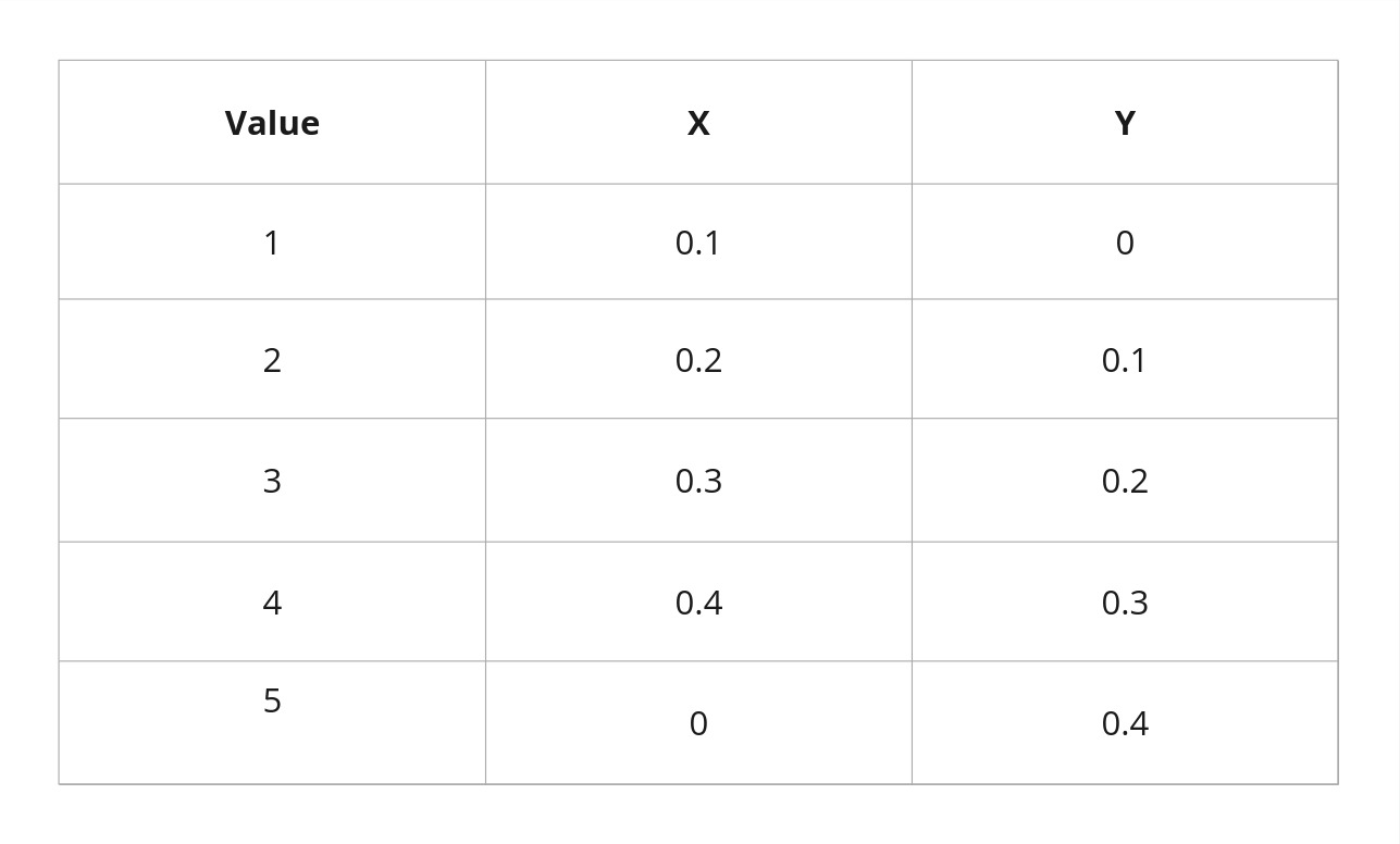
Plotted out, the PMFs of X and Y look like this.

As can be seen, they are not normal. If so, what would the probability distribution of Z look like?

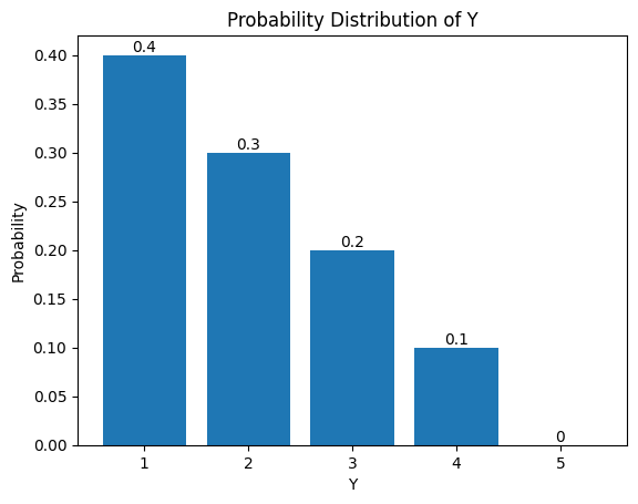
Before we get there, let us go through a couple of examples using the expression for the probability of Z=z.

Say we set Z = 1. Then the probability of Z=1 is zero. This is because if Y = 1 then X has to be zero but that is impossible since X has no chance of being zero (i.e. P(X=0) = 0). The reverse is also true.

Say we set Z = 3. Then there are two scenarios that are possible: 1) X = 1 and Y = 2 and 2) X = 2 and Y = 1. In the first case, we have P(X=1) = 0 and P(Y=2) = 0.1. In the second case we have P(X=2) = 0.1 and P(Y=1) = 0.4. Thus,

\(P(Z = 3) = (0 \times 0.1) + (0.1 \times 0.4) = 0.04\)

Note that X = 3 or Y = 3 is not considered here as it means that the probability of the other variable has to be 0 which in this case is again impossible.

We keep doing this for all possible values of Z to build up its PMF.

The GIF below shows the construction of the PMF of Z using the P(Z=z) equation above. This is done by calculating by brute force the probabilities (see here in the repo).

Construction of the PMF of Z

The more eagle-eyed reader would notice that the construction of Z’s PMF by cycling through possible Z values look like flipping the PMF of Y horizontally and sliding it through the PMF of X. This is actually a mathematical operation called convolution and it will have very interesting consequences as we shall see soon.

z-transforms

Convolution is a very common operation used in signal-processing. It has the interesting property that the convolution of two signals (in our case two PMFs) after being put through certain transformations, such as Fourier Transform, is the simple product of the individual signals after being put through the same transform operation individually. In our case, since our PMFs can be considered as discrete signals, the transform operation that we are interested in is the z-transform.

Suppose, we define

\(\begin{aligned} \mathrm{P}(X=n) &= f(n) \\ \mathrm{P}(Y=n) &= g(n) \\ \mathrm{P}(Z=n) &= h(n) \\ \end{aligned}\)

And the z-transform of a function is denoted by

\(\begin{aligned} \mathrm{Ztransform}(f(n)) &:= \hat{f}(z) \\ &=\sum_{n=0}^\infty f(n)z^k \end{aligned}\)

We use the one-sided z-transform here.

The aforementioned statement can be written as

\(\hat{h}(z) = \hat{f}(z)\hat{g}(z)\)

To make this concrete again, we substitute in the PMFs of X and Y.

\(\begin{aligned} \hat{f}(z) &= 0.1z^2 + 0.2z^3 + 0.3z^4 + 0.4z^5 \\ \hat{g}(z) &= 0.4z + 0.3z^2 + 0.2z^3 + 0.1z^4 \end{aligned}\)

Multiplying the two together, we get

\(\hat{h}(z) = 0.04z^3 + 0.11z^4 + 0.2z^5 + 0.3z^6 + 0.2z^7 + 0.11z^8 + 0.04z^9\)

If we then make the observation that the coefficients of z are actually the values of the PMF of Z at various z values, we can see that we have actually re-produced the PMF of Z here by multiplying two polynomials. This is also a probability generator function.

When things get a little bit more complicated…

Computationally, the case of calculating the PMF of the sum of two random variables is the same in the brute force method and the z-transform method is the same. So what’s the big deal?

The difference comes when you have the sum of more than two random variables. Consider the case of

\(Y = X_1 + X_2 + X_3 \)

The probability of Y = y is

\(\begin{aligned} \mathrm{P}(Y = y) &= \sum_{k_1 = -\infty}^\infty \mathrm{P}(X_1 = k_1)\mathrm{P}(Z=X_2 + X_3 = y - k_1) \\ &= \sum_{k_1 = -\infty}^\infty \mathrm{P}(X_1 = k_1)\sum_{k_2 = -\infty}^\infty \mathrm{P}(X_2 = k_2)\mathrm{P}(X_3 = y - k_1 - k_2) \end{aligned}\)

The above expression is a recursive summation or a nested for-loop (depending on how you implement your code). The more variables there are, the more nested the summation becomes as we have to take into account all the combinations of values that are possible. This is rather undesirable from a computing standpoint.

To take a look at how it would be if we take the transform approach, let’s make the following associations, once again.

\(\begin{aligned} \mathrm{P}(X_i = n) &= f_i(n) \\ \mathrm{P}(\sum_{k=i}^j X_k = n) &= f_{i\ldots j}(n) \\ \mathrm{P}(Y = n) &= g(n) \\ \end{aligned}\)

Then using the definition of the z-transform above, we get

\(\begin{aligned} \hat{g}(z) &= \hat{f_1}(z)\hat{f_{2\ldots 3}}(z) \\ &= \hat{f_1}(z)\hat{f_2}(z)\hat{f_3}(z) \end{aligned}\)

In the above expression, we first treat X2 and X3 as one composite variable (see first row). We then note that the z-transform of (X2+X3) is again the product of the individual z-transforms of the variables.

The reader can convince himself/herself that this works for any number of variables in the sum.

Importantly, if we take the z-transform approach, then the situation becomes one of a product of polynomials which can be done in parallel fashion. Say we have 100 variables we can divide the product in a map-reduce manner to 10 workers that can compute the coefficients of the polynomials separately.